Master querying data in Amazon S3 using SQL (part 1)

Learn how to leverage data formats, partitioning (partition pruning) and predicate pushdown to slash query times and amount of data scanned in Amazon Athena.

Amazon S3 (Simple Storage Service) is a popular choice for storing large amounts of data on AWS. However, efficiently querying this data can be challenging. This article explores various techniques and best practices for querying data stored in Amazon S3.

There are three major components that will be covered in this article:

• Data Store (Amazon S3)

• Data Catalog (AWS Glue Data Catalog)

• Query Engine (Amazon Athena)

Let’s begin…

Data Store (Amazon S3)

Believe me or not, Amazon S3 is not as simple as it’s called.

It’s a mature and feature-rich service that some of the more sophisticated features can surprise even experienced cloud architects. Long story short it’s a scalable object storage service designed to store and retrieve any amount of data from anywhere on the web.

Key Concepts

Amazon S3 uses buckets as containers for objects, with each bucket having a globally unique name. Objects are the fundamental entities stored in S3, consisting of data, a key (name), and metadata. Keys serve as unique identifiers for objects within a bucket. The combination of bucket, key, and version ID uniquely identifies each object.

S3 operates in various geographic regions, where Amazon runs its cloud infrastructure. When creating a bucket, you choose a specific region. This regional approach can help reduce latency, minimize costs, and address regulatory requirements.

It's important to note that S3 doesn't actually have a concept of directories or folders in the traditional sense. What appears as folders in the S3 console are actually prefixes. A prefix is a common string at the beginning of object keys that groups similar objects together. For example, in the key photos/2023/summer/beach.jpg, the prefix would be photos/2023/summer/. This prefix-based organization allows S3 to simulate a folder-like structure, even though it's fundamentally a flat object store. Understanding this distinction is crucial for efficient data organization and querying in S3.

This post accelerates pretty fast, so read along…

File formats

Amazon S3 allows you to store any type of object, but to be able to query it with Amazon Athena, it needs to be structured. There are several types of structured file formats. Let’s list the most popular ones:

• CSV: Simple and widely supported, but inefficient for large datasets.

• JSON: Flexible for semi-structured data, but can be verbose. Usually by JSON people mean JSON Lines — specific format where each line in the file is a valid JSON object.

• Parquet/ORC: Columnar format, highly efficient for analytics workloads.

Columnar formats like Parquet and ORC are generally more efficient for analytical queries, as they allow reading only the necessary columns. This selective column access can significantly reduce I/O and improve query performance. In contrast, row-based formats like CSV and JSON require scanning entire rows, which can be slower and more costly for large datasets.

Columnar formats store data by column rather than by row. This means that all the values for a single column are stored together, allowing for efficient compression and the ability to skip over irrelevant data when querying. This is particularly beneficial for analytical queries that often only need to access a subset of columns.

Data Catalog (AWS Glue Data Catalog)

A Data Lake is a storage repository that holds a vast amount of raw data in its native format. It follows a schema-on-read approach, where the schema is applied when the data is read, not when it's written (like it’s done in the Data Warehouse paradigm). This flexibility requires a schema to be defined at query time.

On AWS, the AWS Glue Data Catalog serves as the central metadata repository for Data Lake (Amazon S3). It stores the schema information that references the location of the data in Amazon S3. The Data Catalog contains databases and tables that define the schema of your data — just like in the typical database, but it doesn’t store the actual data. This metadata is crucial for the query engines to understand the structure of your data and execute queries efficiently.

Query Engine (Amazon Athena)

With data stored in the Data Lake (Amazon S3) and the schema stored in the data catalog (AWS Glue Data Catalog), we can now query the data. To do this, we need an engine to perform read operations and present the data in a structured way using SQL. This is where Amazon Athena comes in.

Amazon Athena is a serverless, interactive query service that makes it easy to analyze data directly in Amazon S3 using standard SQL. It works with various data formats and integrates seamlessly with AWS Glue Data Catalog.

Athena uses Trino/Presto, a distributed SQL query engine, under the hood. This allows it to process large datasets efficiently and quickly return query results.

By leveraging these three components - Amazon S3 for storage, AWS Glue Data Catalog for metadata management, and Amazon Athena for querying - you can build a powerful and cost-effective data analytics solution on AWS.

Querying data in Amazon S3 using SQL

Let's start with a simple example. Assume we have data stored on S3 in JSON Lines format in a directory called data. We have two files: 2024-01.json (10 MB) and 2024-02.json (20 MB), containing records for January and February data respectively.

To query this data, we need to create a catalog that will hold the schema for future SQL queries (schema-on-read, remember?). We can do this easily through the Amazon Athena console by using a CREATE EXTERNAL TABLE statement that references the Amazon S3 bucket. This automatically creates a table in the AWS Glue Data Catalog for us. Here's an example of how this statement might look:

CREATE EXTERNAL TABLE db.events (
  id string,
  type string,
  timestamp string,
  user_id string,
  session_id string,
  status string,
)
ROW FORMAT SERDE 'org.openx.data.jsonserde.JsonSerDe'
LOCATION 's3://your-bucket-name/data/';

Note timestamp column that is going to contain event time, status field and assigned reference location of the data on Amazon S3.

This statement creates a table named events in db database, defining the schema of our data and specifying that it's stored in JSON format in the given S3 location.

Once the table is created, we can query it with SELECT statements referencing the created database and table. For example:

SELECT * FROM db.events
WHERE timestamp >= '2024-01-01 00:00:00'
  AND timestamp < '2024-02-01 00:00:00';

And it works! Now, having the table created, we can perform SQL queries on the objects stored on Amazon S3

However, if you only wan’t to select the data from January than you may notice that you're reading too much data (Data scanned: 30MB). Remember that each query you run in Amazon Athena incurs costs from both Athena’s query charges and the S3 read requests made by Athena. In our example, the query statement should ideally select 50% less — only one file. To achieve this, we need to use a feature called data partitioning.

Data partitioning (partition pruning)

Data partitioning is a technique used to divide large datasets into smaller, more manageable parts based on specific criteria. In the context of Amazon S3 and Athena, it involves structuring the data on S3 in a very specific way, often referred to as Hive partitions.

Hive partitions use a naming convention for prefixes that represents the partition structure. For example, instead of storing data on Amazon S3 as:

s3://my-bucket/data/2024-01.json 
s3://my-bucket/data/2024-02.json

We would structure it as:

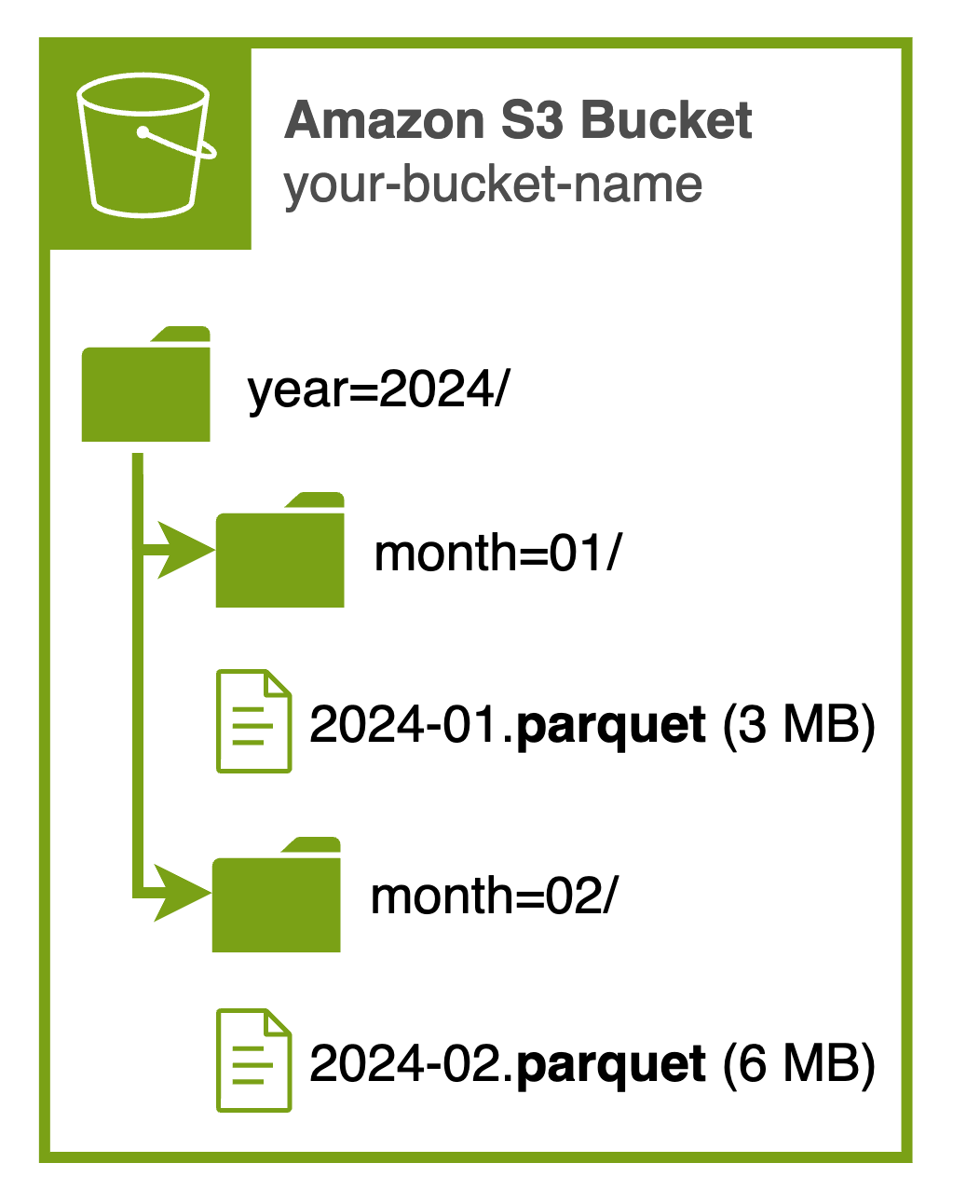
s3://my-bucket/data/year=2024/month=01/2024-01.json
s3://my-bucket/data/year=2024/month=02/2024-02.json

Note that file names doesn’t really matter (shouldn’t) in data processing, so I’m calling it this way just to indicate event data range in each file.

This structure allows Athena to quickly identify which partitions (in this case, which months) it needs to read for a given query, potentially reducing the amount of data scanned and thus lowering costs and improving performance.

To implement partitioning, we need to execute a similar SQL CREATE EXTERNAL TABLE statement, but with an additional clause called PARTITIONED BY. Here's an example:

CREATE EXTERNAL TABLE db.events (
  id string,
  type string,
  timestamp string,
  user_id string,
  session_id string,
  status string
)
PARTITIONED BY (year string, month string)
ROW FORMAT SERDE 'org.openx.data.jsonserde.JsonSerDe'
LOCATION 's3://your-bucket-name/data/';

After creating the table, we need to load the partitions by running the MSCK REPAIR TABLE command:

MSCK REPAIR TABLE db.events;

This command scans the S3 location for Hive partitions and adds them to the table metadata. It’s important to ensure that your table has partitions loaded to return results. You need to add partitions each time you add new data.

Now, when we query the data, we can include partition columns in our WHERE clause to limit the data scanned (just as it would be a column in our data, but it’s a partition):

SELECT * FROM db.events
WHERE year = '2024' AND month = '01';

This query will only scan the data in the year=2024/month=01 partition, significantly reducing the amount of data read from S3 (10MB instead ad of whole 30 MB). Note that we no longer need to use timestamp column to select data by specific year and month!

If we add a day partition, you can further narrow your query by specifying the day. For example, you could target data for January 15, 2024. If you need even more precision, you can also include the timestamp column in SQL query to filter results to a specific time range. For instance, if you want to find events that occurred on January 15, 2024, between 10:00 AM and 2:00 PM.

This approach not only narrows down the data to the specific partition but also allows for finer granularity based on the timestamp, ensuring efficient scanning of only the necessary data, cutting down the cost of each query being executed.

While partitioning can significantly improve query performance and reduce costs, it's crucial to have a balance in your partitioning strategy. Having too many partitions can lead to issues (like having year, month, day, hour, minute… partitions). Too many small files can negatively impact performance due to the overhead associated with opening and closing numerous files. Additionally, excessive partitions increase metadata management in the Glue Data Catalog, potentially slowing down metadata operations. In ideal world, it would be great to keep a file size between 128MB and 2GB (as always, it depends).

Data filtering (predicate pushdown)

While JSON is a flexible format, it's not optimal for efficient querying of large datasets. To take full advantage of advanced querying techniques like predicate pushdown, we should consider switching to a columnar format such as Apache Parquet.

One of the key benefits of using Parquet with Amazon Athena is the ability to leverage predicate pushdown. This optimization technique enables Athena queries to fetch only the data blocks they need (data filter), dramatically improving query performance, time and reducing costs.

Predicate pushdown in Parquet works by using statistics from data block predicates, such as max/min values, to determine whether to read or skip a block. When an Athena query requests specific column values, it can use these statistics to avoid reading unnecessary data.

Let’s assume previous example was written in Parquet instead of JSON.

CREATE EXTERNAL TABLE db.events (
  id string,
  type string,
  timestamp string,
  user_id string,
  session_id string,
  status string
)
PARTITIONED BY (year string, month string)
STORED AS PARQUET
LOCATION 's3://your-bucket-name/parquet-data/';

Now, let's see how predicate pushdown can improve query performance. Suppose we want to find all active events from January 2024:

SELECT id, type, timestamp, user_id, session_id
FROM db.events
WHERE status = 'active' AND year = '2024' AND month = '01';

In this query, Athena uses predicate pushdown in two ways:

1. It only reads the partitions for January 2024, thanks to our partitioning strategy.

2. It only reads the blocks within those partitions that potentially contain 'active' status records, based on the column statistics stored in the Parquet file metadata.

This means that if a particular block's statistics indicate that it doesn't contain any 'active' status records, that block will be skipped entirely, saving both time and processing costs.

By leveraging Parquet format and predicate pushdown, we can dramatically reduce the amount of data scanned and the associated costs, while also improving query performance. This is particularly beneficial when dealing with large datasets where only a small subset of the data is relevant for the query.

Updating the schema and adding new partitions

While creating tables in AWS Glue Data Catalog using Amazon Athena SQL queries works well for static data and demo purposes, it becomes cumbersome when data arrives daily. In such cases, you would need to run MSCK REPAIR TABLE every time you want to load new partitions saved on S3. Moreover, if the schema of the files changes, you'll want to reflect that in the data catalog as well.

Instead of manually managing this process, you can use AWS Glue Crawler. AWS Glue Crawler is a feature of AWS Glue Data Catalog that automatically scans an Amazon S3 bucket, analyzes the data and its partitioning structure, and creates or updates tables for you (both it’s schema and/or partitions).

Here's how a Glue Crawler works:

1. The crawler connects to your data store (in this case, S3).

2. It scans the contents and structure of your data.

3. It creates or updates metadata tables in the AWS Glue Data Catalog.

4. These tables can then be used by services like Amazon Athena for querying.

You can schedule crawlers to run after each data ingestion, which will automatically load partitions to the data catalog, making the data immediately available for queries. This is particularly useful in scenarios where:

• You have frequent data updates

• You process data in incremental batches

• Your data schema evolves over time

• You want to automate the process of keeping your Data Catalog up-to-date

Short disclaimer. I’m not gonna lie, AWS Glue Crawler is a black-box. Sometimes, it’s hard to configure and manage, although it’s relatively easy to setup and automate simple data processing pipeline.

Another way of automatically updating table schema and partitions in AWS Glue Data Catalog could be:

• Use API operations on AWS Glue Data Catalog to add partitions or update schema automatically with your own custom logic and schedule

• Write data using tools that allow you to ingest/write data through the table. For instance, if you're using Amazon EMR or AWS Glue ETL jobs with Spark, you can write your transformed data directly as a table on Amazon S3, and the AWS Glue Data Catalog will be updated automatically. This eliminates the need for separate crawler runs or manual API calls to update partitions or schema changes. (but, thats a topic for another article)

Key takeaways

1. Use columnar formats like Parquet for better performance

2. Leverage AWS Glue Data Catalog for metadata management

3. Implement data partitioning to reduce data scanned, but keep the balance

4. Utilize predicate pushdown for optimized queries (Parquet format does it for you)

5. Automate metadata management for incremental data. For example with AWS Glue Crawlers

There is one more thing (or even more)… Table Formats such as Apache Iceberg and Apache Hudi, but that's coming in part 2 of this article!

Subscribe to motivate me to finish part 2… and receive email about it.